New Apartment Loan Amortizationsummit Create An E
- Select the Search worksheet and then the Pet Deposit column. Create a formula to determine the required pet deposit for each unit. If the unit has two or more bedrooms and was remodeled after 2006, the deposit is $150; if not, it is $100.
- The Recommendation column needs a nested function to indicate the remodeling status. If the apartment is unoccupied and has not been remodeled before 2006, then display “Please remodel” in the Recommendation column. Display ” ~ No Change” for apartments that do not meet the former criteria.
- Make sure each field has the appropriate professional formatting for titles, headers, currency, percent, and so forth. Your worksheets need to be readable, clean, and professional. Please let spell-check work for you; use this feature to check for spelling errors.
Click Image to Expand
Step 2: Quick Search
Now that all of the rental properties are listed and organized, the owners would like to be able to search through the apartment numbers and return the price of the apartment number listed.
- Insert number 1301 in cell B3. B3 is the cell that will be used to research apartment unit prices.
- Create a nested lookup function in cell E3. Look up the rental price in column D using the apartment unit number in cell B3. (Use the INDEX function.)
- Make sure each field has the appropriate professional formatting for titles, headers, currency, percent, and so forth. Your worksheets need to be readable, clean, and professional. Please let spell-check work for you; use this feature to check for spelling errors.
Click Image to Expand
Step 3: New Apartment Loan Amortization
Summit Ridge Ski owners want to purchase a sixth apartment complex. This decision is under review. Here are the details of their offer. The loan amount is $950,000 with a down payment of $400,000 for 30 years at 5.325%, with the first payment due on January 20, 2017. Please consider the loan calculations and build a loan amortization table on the Loan worksheet. Click on the Loan worksheet to begin.
- In the Loan area (A1 through E7), enter the loan details in the Input Area based on the information provided above. Place formulas to create all calculations in the Summary Calculations. The loan payment is at the end of the period.
- Create a loan amortization table with the header row in A10 through F10. Add payment # (1 thru 360 for a 3-year loan). Use autofill to help. The Payment Date column needs a date function. The Interest Paid and Principal Payment columns require financial functions.
- Format the sheet professionally and create a custom footer with your name on the left side, the page and page number in the center, and your professor’s name on the right side of each worksheet. Make sure you put the page back to normal view after you insert the footer at the bottom.
Step 4: Conditional Functions
In addition to adding the new apartments to their financial portfolios, the owners of Summit Ridge Ski Resort would like to ensure that they are paying their employees at market value and want to continue to encourage employees to stay with the company. Another phase of your project is to research all employee salaries to see if they have any effect on job satisfaction. Employee satisfaction surveys allow the company to get a pulse for how content employees are. A voluntary survey was administered to a cross-section sample of all employees in the company. This next bit of work will be on the Employee Satisfaction Worksheet.
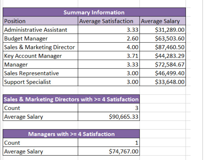
- Calculate the average job satisfaction for Administrative Assistant in cell H5. Format the results with the number format and two decimal positions.
- Use the fill handle from cell H5 to copy the function down through the range H6:H11. Make certain to consider the appropriate mixed and/or absolute cell referencing.
- Calculate the average salary of all Administrative Assistants and place the result in cell I5.
- Use the fill handle from cell I5 to copy the function down through the range I6:I11. Make certain to consider the appropriate mixed and/or absolute cell referencing.
- Calculate the number of Sales and Marketing Directors in cell H14 that have a job satisfaction level of 4 or above.
- Calculate the average salary of Sales and Marketing Directors in cell H15 that have a job satisfaction level of 4 or above.
- Use a process like that demonstrated in steps E and F to calculate the total number and the average salary of Managers that have a job satisfaction of 4 or greater.
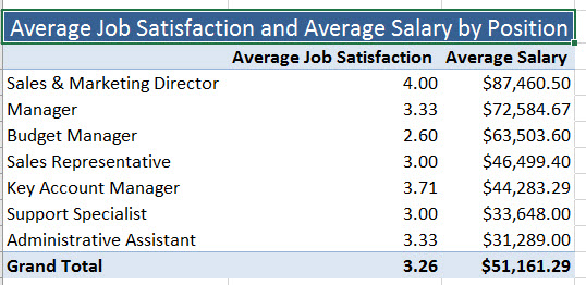
H. Use the Employee Satisfaction data to create a Pivot Table showing the average salary and Job Satisfation by Position (rows). Format professionally and sort highest salary to lowest.
Step 5: Create a Documentation Sheet
Clean up the formatting of your Excel workbook, taking into account professional appearance.
The Minimum Requirement (per the Grading Rubric)
- Insert a new spreadsheet into the workbook. The Documentation sheet should be the first sheet in the workbook.
- Make certain each tab has a descriptive name and color for each tab (sheet) in the workbook.
- Create the professional documentation worksheet. Be sure to include a description of each worksheet. An image is provided below.
Finish and Submit
Save your Excel file. Make sure you are aware as to where your files are physically saved. Saving your file often is good practice (Ctrl + s).
Your Excel file should contain five worksheets.
- Documentation Page
- Search
- Loan
- Employee Satisfaction
- Satisfaction Pivot Table
Submit one workbook. When submitting the workbook, provide a comment in the comments area explaining what you learned from completing this lab activity. File naming convention: If your name is Jane Doe, then your file should be named very similar to Doe_J_Week5_Lab.xlsx.


